Importing database dump files with impdp

In this guide, we'll cover how to import a DMP file into an oracle database using impdp:

Creating sample data viz and dashboards is a common request when we talk about 'the art of the possible'.  If we're lucky, we can use the "Sample Sales" data set provided OOTB with OBIEE and OAC. Since the beginning of OBIEE time, Sample Sales has served us well. Fast forward to 2018, we're seeing an increase in demos and proof of concepts with client/customer data, and it's not in excel files anymore.

We're getting data sets which are database extracts, commonly called DUMP files.   It's a single file representation of an entire data set within a schema, including tables, fields, permissions and the actual data. Importing dump files into an oracle database can be done via datapump the command line 'impdp'.

Here's how to import a dmp file to an Oracle 12c database. We'll be using command-line sqlplus and an  oracle 12c database which are both in a virtual machine running Oracle Linux. This can also be done using the Data Pump Import Wizard using SQL Developer.

Step 1. Know your database directories 

I found this to be the most common point of failure when importing data via impdp.  Know the dba directories within your oracle db by running. Make sure you're logged in as sysdba:

sqlplus sys as sysdba;
select * from dba_directories;

Step 2. Create and grant applicable privileges

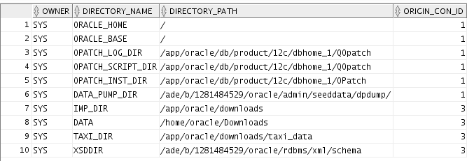
CREATE USER BISAMPLE IDENTIFIED BY Helloworld123;

Creates a schema BISAMPLE with password Helloworld123.

GRANT CONNECT, RESOURCE, DBA TO BISAMPLE;

We are assuming that this user is a power user that can:

1. Allows the user to connect and query the BIDEMO schema (connect)
2. Allows the user to create named types for custom schemas (resource)
3. Allows the user to not only create custom named types and alter and destroy them as well (DBA)

8.  GRANT READ, WRITE ON DIRECTORY DATA TO BIDEMO;

Gives BIDEMO user access to dba_directory 'data', in this example its located at /home/oracle/downloads

Step 3. Import the dump file

    impdp system@orcl full=y directory=DATA dumpfile=BISAMPLE.DMP

Running impdp via command line as outlined above will import the BISAMPLE.dmp file located in /home/oracle/downloads to the schema BISAMPLE.

Step 4. Verify the import

Take a second to log in as the user we created (BISAMPLE) and verify that the quantity of tables we imported are actually in the schema

    sqplus BISAMPLE;
select table_name, status, num_rows from USER_TABLES;

In this import we expect to see 62 tables added to the BISAMPLE schema as verified below

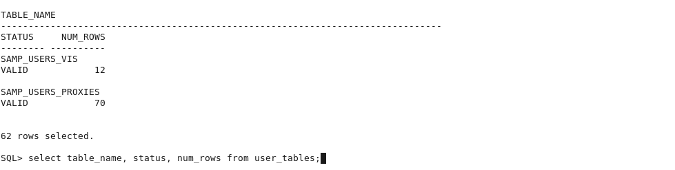
Now we can use the awesome capabilities of Oracle Analytics to connect to this db to perform mash ups, analytics and advanced data viz! I know alot of you guys were asking this as a follow up to our earlier post on creating a shared folder w/in an Oracle Linux Virtual Box.  This post should help. Now you can:

1. Create or receive a DMP file on your host machine, or via another user
2. Transfer the DMP file to the target machine which contains the isolated oracle database
3. Use the OBIEE 12c publically available image to create interactive reports, dashboards, data viz, and more! 

Happy demoing!

Create a shared folder with an Oracle Linux VirtualBox + Windows 10

With the release of the OBIEE 12c virtual appliance  there's plenty of opportunity conduct demo days, proof of concepts and daily-in-the-life scenarios for your customers and stakeholders. A recurring challenge we continue to hear is the ability to upload custom data sets or BAR files within the VM.

Friendly reminder that the VM is an encapsulated 'machine-in-a-box' that has no network connectivity to your local machine (the host). To enable file sharing between your Virtual Machine and your host, remember to create a shared folder. There's some confusion on how to do this, so we'll explain as follows.

Keep in mind, the 'host' is your local machine, the 'guest' is the virtual machine, and the 'mount' is the shared folder between the host and guest. In this example, the host is a windows 10 machine provisioned by a client, and the guest is the OBIEE 12c v607 Virtual Appliance VM (Oracle Linux) installed on the host accessed via VirtualBox.

Step 1. Identify a folder to share on your host machine.

In this case we'll create a folder in our C:\ drive called shared_vm

Step 2. Add the shared folder to the VirtualBox share

Within your Oracle VirtualBox VM setting navigate to shared folders and mount C:\shared_vm. This tells the VM that C:\shared_vm is the shared folder on the host.

Step 3. Insert the Guest Additions CD Image within the VirtualBox

This is where alot of people fail. I've seen numerous blogs and youtube videos where people attempt to run the guest addition CD image on the host. Guest Addition = guest machine. Do not run the image on the host (windows), run it within Virtual Machine (in this case Oracle Linux). 

By running Devices -> Insert Guest Images CD, you'll be prompted with a selection to 'Open Autorun Prompt'. Not you'll be required required to enter the root password for this image which is 'Admin123'. This isn't a secret, all user/passwords within the appliance are accessible via the default link within firefox.

You'll be prompted with a notification that modprobe vboxsf has failed. modprobe is a function to add or remove module's from the linux OS kernel. 

Execute

sudo usermod -aG vboxsf $(whoami)

to add the logged in user to the vbox group, then restart the server. 

Step 4. Create a shared folder within the guest machine and mount to the virtualbox shared folder

In this example we created a folder called 'shared' in /home/oracle. 

Mount the virtualbox shared folder (called "shared_vm" which was created step 2) to /home/oracle/shared by executing

sudo mount -t vboxsf -o uid=1000,gid=1000 shared_vm /home/oracle/shared

To verify, we created a file  in our host location c:\shared_vm which is also visible in the guest folder /home/oracle/shared

Happy demoing!

How-to: Upgrade Usage Tracking OBIEE 10g to OBIEE 11.1.1.x

Oracle has provided plenty of documentation on how to upgrade your OBIEE 10g environment to their new 11g platform. They've even outlined the process of configuring a new instance of Usage Tracking on a new 11g environment - outlined here. What I haven't been able to find is the ability to take an existing Usage Tracking environment in OBIEE 10g, and port it over to the new 11g environment. The upgrade assistance tool won't work because the data model for Usage Tracking has actually changed between the two versions.  This guide is going to cover the process of:

• Taking an existing OBIEE 10g Usage Tracking environment 
• Making the necessary changes to the Usage Tracking data model
• Applying the configuration changes in weblogic to enable Usage Tracking in OBIEE 11g

Step 1: Make changes to existing OBIEE 10g Usage Tracking RPD

The data types and nullable check box have changed for nearly every column in Usage Tracking's primary table: S_NQ_ACCT. Using the Admin Tool, modify each column as outlined below:

Step 2: Modify Physical Data Model

I've noticed on some engagements that the NQ_LOGIN_GROUP table may not always be deployed. I don't think this is an 'out of the box' table but rather something manually deployed to track the applicable group of an individual user. Note that as you move to the application role based security model you'll no longer need this table. In the event that you do need this backwards compatibility, you'll need to fix the broken link - which is made evident by the red line that appears when you attempt to display the physical data model:

You'll need to make the physical join on NQ_LOGIN_GROUP.LOGIN = S_NQ_ACCT.USER_NAME

Step 3: Enable Usage Tracking in Enterprise Manager

It's at this step where Usage Tracking implementation differs dramatically between OBIEE 10g and OBIEE 11g. In the 10g platform, Usage Tracking was enabled by modifying the nqsconfig and instanceconfig files, but with the advent of Oracle's Enterprise Manager you must now go through EM's MBeans configuration to enable the tool.  To Oracle's credit, they did provide a detailed guide on how to enable Usage Tracking in EM . Rather than re-invent the wheel, i'm going to defer everyone to the section titled 'Configuring Usage Tracking in Enterprise Manager'. We're past the 'OBIEE 10g' upgrade so Oracle's guide is more than appropriate.

Step 4: Deploy Usage Tracking Tables to Your 11g Database

Most implementations use the DEV_BIPLATFORM that come pre-populated with the S_ETL_DAY, S_ETL_TIME_DAY and S_NQ_ACCT tables, but if your version did not, or you're not using the default schema, run the following scripts located at the following directory:

instances\instance1\bifoundation\OracleBIServerComponent\coreapplication_obis1\sample\usagetracking\

1. Oracle_create_nQ_Calendar.sql
2. Oracle_create_nQ_Clock.sql
3. Oracle_nQ_Calendar.sql
4. Oracle_nQ_Clock.sql

Step 5: Confirm Usage Tracking is Enabled

I've created a sample report with the Usage Tracking subject area as outlined below:

 

When viewing the log generated by the query, you'll see that a query is generated against the Usage Tracking connection pool and no error is thrown!



 

keywords: obiee 11g, usage tracking,  upgrade usage tracking , enterprise manager

 

How-to: Automated Web Catalog Deployment in OBIEE 11g

In a previous article I covered the process of how to automatically migrate the repository from a developer environment to production. Equally important is the process of migrating the web catalog.  Most BI Architects are familiar with the ability to archive and unarchive, but there are many unknowns that the Oracle documentation does not cover.

• What about version control?
• How do you migrate only select files?
• How do you migrate object level security?
• What if there are multiple people editing the web catalog?

A typical web catalog migration path consists of:

1. Developer checks out or download a local copy of the web catalog from version control
1. This is only done on an as needed basis
2. Developer makes changes to specific web catalog files
3. Developer archives changes
4. Developer checks out a folder (in this case called archive.zip) from version control that contains all production changes for the specific release
5. Developer adds their changes to the archive.zip
6. Developer updates 'change list' within the archive.zip to contain path of changed document
7. Developer checks-in archive.zip to version control
8. Deployment script automatically propagates through out each environment as outlined below:

This process uses the 'archive.zip' file as the directory to propagate changes throughout all environments. This is a preferred method because the archive.zip file only contains changes to the web catalog, and not the entire web catalog itself.

What's in the archive.zip?

The archive.zip will contain 

1. Only the modified web catalog objects for your specific release. 
2. A csv file that contains the destination path of each web catalog object
1. This is used as input for the shell script we're going to create for automatic deployment
2. I call this file 'Catalog_Deployment.csv' but it can be renamed if needed

Your archive.zip file might contain the following:

In the above example I have 5 files:

1. Financial_Reports.catalog is an archive of the 'Financial Reports' folder which contains multiple reports
2. Financial_Reports_Dashboard.catalog is an archive of the Financial Reports Dashboard that displays all of the financial reports
3. HR_Reports.catalog is an archive of the 'HR Reports' folder which contains multiple reports
4. HR_Reports_Dashboard.catalog is an archive of the HR Reports Dashboard that displays all of the HR reports
5. Catalog_Deployment.csv is a csv file that contains the target directory path when we unarchive each catalog file (via a shell script)

In the above example, the Catalog_Deployment.csv file would contain the following:

The Catalog_Deployment.csv contains only 2 columns:

1. The name of the archive file(s) in your archive.zip (Column A)
2. The unarchive target directory (Column B)

How do you identify the unarchive target directory (Column B)?

The unarchive target directory (column b) can be found in the 'location' section of the' properties' tab for the specific folder you're trying to archive:

Let's cover the steps required in order for the web catalog to make it out of the developer's box and into assembly test

Step 1.  Check out the archive.zip file from your version control software

'Check out' is the correct terminology because this will ensure the file is locked and no one can make any changes except for the specific developer. You should now have a locked version of archive.zip that you can modify.

Step 2. Archive the modified web catalog files

This is a straight forward step that can be achieved through Answers. The archive button can be found in the 'tasks' section as noted below:

Step 3. Modify the archive.zip file & Re upload to Version Control

Your modifications should include:

1. The addition of the modified .catalog files
2. Revisions to the Catalog_Deployment.csv 

Once the changes are made, you can upload back to Version Control and 'check the archive.zip' back in so other developers can add their changes. The key here is only one developer modifies the archive.zip file at a time!

Step 4. Pragmatically deploy the web catalog via a deployment shell script

The script we're going to use is going read each row in the Deployment_Catalog.csv file and and use Catalog Manager's runcat.sh script to perform command line based unarchiving.  Oracle has very little documentation on runcat.sh, but think of it as a way to launch Catalog Manager. You can launch Catalog Manager in either GUI mode or command line mode. Using the '.runcat.sh -cmd unarchive' parameters, we're telling Catalog Manager to unarchive in command line mode.

#!/bin/bash
#
# This file will read the archive files that are unzipped in /tmp/webcatmigration
#

/bin/dos2unix /tmp/webcatmigration/archive/Catalog_Deployment.csv /tmp/webcatmigration/archive/Catalog_Deployment.csv1
rm /tmp/webcatmigration/archive/Catalog_Deployment.csv
mv /tmp/webcatmigration/archive/Catalog_Deployment.csv1 /tmp/webcatmigration/archive/Catalog_Deployment.csv
while IFS=, read file path
do
echo ""
echo First Column in Catalog_Deployment - $file
echo Second Column in Catalog_Deployment - $path
echo ""
/export/obiee/11g/instances/instance1/bifoundation/OracleBIPresentationServicesComponent/coreapplication_obips1/catalogmanager/runcat.sh -cmd unarchive -offline /export/obishare/catalog/webcatalog -inputFile /tmp/webcatmigration/archive/$file -folder "$path"
done < /tmp/webcatmigration/archive/Catalog_Deployment.csv
~

This script does the following:

• Converts the .csv file from binary to unix via dos2unix
• Reads each row in Catalog_Deployment.csv and passes A(N) and B(N) for each row to the $file and $path parameters

A good option for automatic deployment would be to have this script run every Friday after hours as part of the deployment process. You would have one script in each environment for deployment. Ideally the script would be able to read directly from the file server of your version control software.

In summary, we've accomplished the following:

• Implemented a mechanism to manage web catalog modifications
• Automated the web catalog deployment process
• Minimized human error

Notes

How often should I back up the entire web catalog?

Notice that the only component of the web catalog being uploaded to version control are the actual changes to the web catalog objects. It is a good idea to take a back up of the entire web catalog prior to the 'go live' of deployment of each 'new release'

What about object level security?

The runcat.sh and archive/unarchive functionality will automatically migrate object level security of each object, but if the object level security is using new application roles that do not exist in the assembly/system/pre-production/production environments - the application roles must first be created in each environment's Enterprise Manager.

Don't forget about the GUIDs!

If you are migrating to a production environment that has different authentication providers than the non-production environment(s) - you must refresh the GUIDs first. You can read how to refresh the GUIDs in this Oracle note - How to refresh GUIDs for OBIEE 11g ? (Doc ID 1564006.1)

 

keywords: OBIEE 11g, deployment, archive, unarchive, migration, answers, runcat.sh web catalog, webcat

How-to: Bridge Tables and Many to Many Relationships Demystified in OBIEE 11g

Bridge tables - entire books have been devoted to this concept, countless blogs write about it, and organizations offer entire classes dedicated to demystifying this idea. Ralph Kimball, creator of Kimball Dimensional Modeling and founder of the Kimball Group has written quite a few great articles discussing the theory of bridge tables.

Yet when researching for comprehensive guides on how to actually implement a bridge table in OBIEE 11g, the documentation available is either:

• Out of date
• Contains implementation steps for OBIEE 10g which has since been deprecated
• Does not contain adequate detail 
• e.g. missing key steps

This guide is going to outline the basic use case of a many to many relationship, how OBIEE 11g resolves this dilemma and how to successfully implement a bridge table model within the 11g platform.

First thing's first - what is a bridge table and why do we need it?

At its core, bridge table solve the many to many relationship we encounter in many datasets. Many to many relationships in itself are not "bad", but when attempting to conform a data set to a star schema - many to many relationships just do not work. Star schemas assume a one to many (1:N) cardinality from the dimension to the fact. This means "one attribute of a dimension row can be found in many rows of the fact table".

For Example:

• One job (job dimension) can be performed by many people
• You would see the same JOB_WID repeating in the fact table
• One employee (employee dimension) can have many jobs
• You would see the same EMPLOYEE_WID  repeating in the fact table
• One call at a call center(ticket dimension) can have many ticket types
• You would see the same CALL_WID repeating in the fact table
• One patient (patient dimension) can have many diagnosis
• You would see the same PATIENT_WID repeating in the fact table

This 1:N cardinality is represented in OBIEE as (using call center/employee example) :

"Cardinality of '1' applied to the dimension and cardinality of 'N' applied to the fact'

But what happens when in the above examples, the cardinality is actually N:N? 

For Example:

• Many employees can have multiple jobs and each job can be performed by multiple employees
• Many patients can have multiple diagnosis and each diagnosis can be 'assigned' to many patients
• Many calls can have multiple call ticket types and each ticket type can belong to multiple calls

This many to many relationship is initially (and incorrectly) represented in OBIEE 11g as:

'Cardinality of '1' is applied to the two dimension tables and cardinality of 'N' is applied to the fact'

Any BI Architect should recognize the above model - it's a traditional star schema! If you stop here and decided to ignore the issue with your dataset and 'hope' OBIEE aggregates the model correctly, you're about to be disappointed.

Why star schemas dont work for N:N cardinality

Consider the following scenario: You're a call center manager and you want to capture the number of calls with positive feedback per employee. You also want to capture the type of calls an employee answers in any given day.

Upon analysis of the requirements you conclude that "each call received by an employee can have many call types and each call type can be answered by multiple employees".

For example:

• I answer a take a call that is classified as a 'new call', 'urgent', and 'out of state transfer' (three different call types) - this is the "each call received by an employee can have many call types".
• A colleague also received a phone call that is classified as 'out of state transfer' - this is the 'each call type can be answered by multiple employees"

Now let's put this data in a traditional star schema fact table as modeled below:

ID	EMPLOYEE_WID	CALL_TYPE_WID	NUMBER_OF_GOOD_CALLS
1	1	1	300
2	1	2	300
3	1	3	300
4	2	2	500
5	2	3	500
6	3	1	200

You can see in the above data set that:

• EMPLOYEE 1:
• Has 3 different call types
• Has 300 positive reviews (NUMBER_OF_GOOD_CALLS) 
• This metric is at the EMPLOYEE level and not the call type level!
• EMPLOYEE 2:
• Has 2 different call types
• Has 500 positive reviews (NUMBER_OF_GOOD_CALLS)
• This metric is at the EMPLOYEE level and not the call type level
• EMPLOYEE 3:
• Has 1 different call type
• Has 200 positive reviews (NUMBER_OF_GOOD_CALLS)

Now you receive a requirement to create a KPI that displays the Number of Good Calls as a stand alone widget.

PROBLEM 1 - Aggregation :

The number of good calls you received based on the above fact table is not 2100 - it's 300 + 500 + 200 = 1000

• Employee 1 received 300 good calls
• Employee 2 received 500 good calls
• Employee 3 received 200 good calls

but due to the many to many cardinality of the data, the star schema duplicates the measures because each employee can take calls of many call types and each call type can be assigned to many employees!

PROBLEM 2 - Grand Totaling:

What if you don't care about aggregates? What if you just want a report that contains the employee, call type and a summation/grand total?

Notice how NUMBER_OF_GOOD_CALLS is repeated across multiple call types and the grand total is still incorrect. It's being duplicated due to the many to many relationship that exists between call type and employee. Furthermore, it paints an incorrect picture that NUMBER_OF_GOOD_CALLS is some how related to CALL_TYPE

How do we resolve this many to many cardinality with a bridge table?

When all is said and done, the incorrectly built star schema:

should be modified to:

Let's break this down:

The bridge table:

This the purpose of the bridge table is to resolve the many to many relationship between the call type and employee. It will contain, at a minimum, the following four columns:

1. The primary key of the table
2. The EMPLOYEE_WID
3. The CALLTYPE_WID
4. The weight factor

The weight factor is what's going to resolve the issue of double counting. 

• If an employee has 3 call types, there would be 3 rows and the weight factor of each row would be .33
• If an employee has 10 call types, there would be 10 rows and the weight factor of each row would be .1

In our bridge table data set, we're going to use the same 3 EMPLOYEE_WIDs and create the following:

ID	CALL_TYPE_WID	EMPLOYEE_WID	WEIGHT
11	1	1	0.33
12	2	1	0.33
13	3	1	0.33
23	2	2	0.5
24	3	2	0.5
31	1	3	1

You can see from this example that we've taken the N:N dataset in the fact table and moved it into this bridge.

The dimension that is joined to both the fact and bridge

This is a generic dimension that contains the unique EMPLOYEE IDs in your organization's dataset.

For example:

ID	EMPLOYEE_ID
1	1
2	2
3	3
4	4
5	5
6	6
7	7
8	8
9	9
10	10

The dimension that is joined to only the bridge table

This dimension contains all of the possible call types. Note how this table is not physically joined to the fact. This is because this specific dimension (CALL_TYPE) is what's causing the N:N cardinality

For example:

ID	DESC
1	Call Type 1
2	Call Type 2
3	Call Type 3
4	Call Type 4
5	Call Type 5
6	Call Type 6
7	Call Type 7
8	Call Type 8
9	Call Type 9
10	Call Type 10

The Fact Table

We've moved the N:N cardinality from the original fact table to the bridge table so the new fact table now contains exactly one row per employee and does not have the CALL_TYPE_WID.

ID	EMPLOYEE_WID	NUMBER_OF_GOOD_CALLS
1	1	300
2	2	500
3	3	200

How do we implement this model in OBIEE 11g?

Step 1: Import Tables into Physical Layer

This is always the first step performed when creating a model regardless of its type. In the above example i'm importing four tables:

Step 2: Create the Physical Data Model

Based on our data set above the join conditions would be implemented as follows:

• 1:N relationship from employee dimension to fact table
• 1:N relationship from employee dimension to bridge
• 1:N relationship from call type dimension to bridge

Notice how employee_demo_d is the only dimension that is joined to the fact. w_call_type_d is not joined to the fact because that is the dimension that is causing the many to many relationship issue.

Step 3:  Create the Logical Data Model
The creation of the BMM is where we deviate from our standard build steps of a traditional star schema:

1. All associated dimension tables referencing the bridge table will be stored in a single BMM table
2. The single BMM table will have two logical table source

Step 3.1 : Drag the fact table and dimension table that is connected to the fact table into the BMM. 

In our example, we are dragging w_calls_f and w_employee_demo_d into the BMM:

Step 3.2: Create a 2nd LTS in the existing dimension table

1. Right click W_EMPLOYEE_DEMO_D -> New Object -> New Logical Table Source
2. Name it 'Bridge'
3. Add W_BRIDGE_D and W_CALLTYPE_DEMO_D (the two dimensions not directly joined to the fact table) under the 'Map to these tables' section

1. Next add the remaining dimension columns from W_CALLTYPE_DEMO_D and W_BRIDGE_DEMO_D to the Dimension table in the BMM

Step 3.3: Create a level-based dimension hierarchy for the dimension BMM

1. This step should be completed whether or not the schema is a star or bridge

Step 3.4: Confirm the BMM model has a 1:N relationship from the dimension to fact

Step 3.5: Set aggregation rule of NUMBER_OF_GOOD_CALLS to sum 

All measures in the BMM must have a mathematical operation applied to the column

Step 3.5: Set the Content level of the dimension table to 'detail' in within the LTS of the fact table

Again, this is something that should always take place regardless of the type of model

Step 4: Create the Presentation Layer

This part is straight forward, just drag the folders from the BMM into the new subject area:

The moment of truth

So why did we go through this elaborate exercise again? To fix the aggregation issues we were having with NUMBER_OF_GOOD_CALLS due to the N:N cardinality of the data set. Let's create that 'standalone KPI' Number of Good Calls:

Notice how the metric correctly sums to 1000. Let's check the back end physical query to confirm:

Notice how it's hitting the fact table and not the bridge or the call type dimension. 

But what about the weight factor?

Let's go back to the scenario where we want to compare across dimensions joined via the bridge table (EMPLOYEE and CALL_TYPE):

• When creating a report that uses a measure from the fact table, a dimension value from the the employee table, and a dimension value from the table that causes the N:N cardinality - you need to use the weight factor to make sure your measure isn't getting double or triple counted:

• Notice column is using the the NUMBER_OF_GOOD_CALLS multiplied by the WEIGHT factor in column 2
• Each row in column 1 correctly represents the NUMBER_OF_GOOD_CALLS in the fact table despite having the repeated values of multiple call types
• Note the aggregation of grand total sums to 997. This is because the weight factor is rounded to the 2nd decimal for EMPLOYEE_WID = 1 (.33%)

In order for grand totaling to work correctly with bridge table measures that use weight facts you must set the aggregation rule of the column (in this case column 1) to sum within Answers:

So what did we accomplish in this guide?

• A basic understanding of many to many (N:N) cardinality
• A basic understanding of why the star schema won't work for N:N cardinality
• How to resolve the cardinality issue with a bridge table
• How to implement a bridge table in OBIEE 11g

keywords: bridge table, cardinality, many-to-many, OBIEE 11g, helper table, answers, analytics, aggregation, LTS, measures, kimball

FYI: GoURL Primer with OBIEE 11g

The Oracle BI Presentation Services Go URL command is for use in incorporating specific Oracle Business Intelligence results into external portals or applications. The Go URL is used when you add a result to your favorites, or add a link to a request to your dashboard or an external Web site. It has a number of forms and optional arguments that can be used to control its behavior.

Oracle has provided limited documentation on goURL parameters and with use cases that require end users to navigate to specific dashboards or request dashboards be embedded into pre-existing web pages, i've decided to create a Primer on commonly used GoURL functionality:

Common goURL Parameters:

Parameters	Syntax	Definition
NQUser	&NQUser=x	User ID
NQPassword	&NQPassword=x	Password
Path	&Path=x	Path of the answer to execute. You can find it in the properties page (Answers/Manage Catalog/ and click on the properties icon (a little hand) of the object that you want. See picture above
Link Options	&Options=x	The x can be one or more of the following letters: * m : Modify Request * f : Printer Friendly * d : Download to Excel * r : Refresh Results
Printer Friendly	&Action=print	Results are in a printer-friendly format, without the paging controls, hot links, and so on.
Passing Filters	&Action=Navigate	To apply filters to the answer (see section below on Passing Filters)
Application Friendly	&Action=Extract &Action=Scroll	Results are displayed in an application-friendly format, such as for Microsoft Excel, without the paging control, hot links, and so on. The Extract action also acts as a Navigate action (read Passing Filters to the Oracle BI Presentation Services Go URL Through a URL (Navigation)) so you can filter the results that are returned by the call.
Specific View	&ViewName=x	This shows an individual result view rather than the default compound view
Specific View	&ViewID=go~x	This shows an individual result view rather than the default compound view where x is the name of the view
Specific Style	&Style=x	This shows the results using a specified style. If the style does not exist, the default is used.
Result Format	&Format=x	This controls the format of the results. This is the format, where x can be xml, html, txt (tab separator), csv (comma separator)
File Extension	&Extension=.csv	This controls the file extension of the download file
Language	&Lang=fr	This controls the language of the report. The value permitted are the values of weblanguage
done	&done=portalPages	parameter allows you to create a return link equal to a path that you have specified

Passing Filters

You can use the &Action=Navigate in conjuction with the with the parameters below to pass filters directly to a report via goURL. Use &P0=n where n equals the number of parameters you wish to filter and P1...to P6 with the one or more of the operators below:

Operator	Meaning
eq	Equal to or in.
neq	Not equal to or not in.
lt	Less than.
gt	Greater than.
ge	Greater than or equal to.
le	Less than or equal to.
bwith	Begins with.
ewith	Ends with.
cany	Contains any (of the values in &P3).
call	Contains all (of the values in &P3).
like	You need to type %25 in place of the usual % wildcard. See the examples that follow.
top	&P3 contains 1+n, where n is the number of top items to display.
bottom	&P3 contains 1+n, where n is the number of bottom items to display.
bet	Between (&P3 must have two values).
null	Is null (&P3 must be 0 or omitted).
nnul	Is not null (&P3 must be 0 or omitted).
&P2=ttt.ccc	In this parameter, ttt is the table name and ccc is the column name. If the table or column contains spaces, it must be quoted with double-quotes.  Spaces should be escaped as %20, for example, Measures."Dollar%20Sales".
&P3=n+xxx+yyy+...+zzz	In this parameter, n is the number of values, and xxx, yyy, and zzz are the actual values. Note: If the value of P3 begins with a numeric character, the entire value must be enclosed in quotes. example: saw.dll?Go&Path=/Shared/Test/SB2&Action=Navigate&P0=1&P1=top &P2=Customers.Region&P3="7

Passing Filters Examples:

his returns records for the East and Central regions:

Saw.dll?Go&Path=/Shared/Test/SB2&Action=Navigate&P0=1&P1=eq&P2=Customers.Region&P3=2+Central+East

This returns records for like Regions E....t:

saw.dll?Go&Path=/Shared/Test/SB2&Action=Navigate&P0=1&P1=like&P2=Customers.Region&P3=1+E%25t

This returns the top two regions by dollars sold:

saw.dll?Go&Path=/Shared/Test/SB2&Action=Navigate&P0=1&P1=top&P2="Sales%20Facts".Dollars&P3=1+2

This is an example where the number of arguments is not included in the syntax:

saw.dll?Go&Path=/Shared/Test/SB2&Action=Navigate&P0=1&P1=top&P2=Customers.Region&P3=Central

This returns records with between 2,000,000 and 2,500,000 in sales:

saw.dll?Go&Path=/Shared/Test/SB2&Action=Navigate&P0=1&P1=top&P2="Sales%20Facts".Dollars&P3=2+2000000+2500000

This returns records for Regions beginning with the letter E:

saw.dll?Go&Path=vate&P0=1&P1=bwith&P2=Customers.Region&P3=1+E

This returns records for Regions containing the letter E and having more than 20 million in sales:

saw.dll?Go&Path=/Shared/Test/SB2&Action=Navigate&P0=2&P1=cany&P2=Customers.Region&P3=1+e&P4=gt&P5="Sales%20Facts".Dollars&P6=1+20000000

Generating SQL Statements using goURL:

The Go URL command can be used to issue Oracle Business Intelligence SQL. These forms of the Go URL return tabular results. The basic options from &Style= and &Options= can be used here as well.

To issue Oracle Business Intelligence's simplified SQL, include the escaped SQL as a parameter to the Go URL. For example:

saw.dll?Go&SQL=select+Region,Dollars+from+SupplierSales

where the FROM clause is the name of the Subject Area to query.

Alternatively, the command IssueRawSQL can be used to bypass the Web processing and issue SQL directly against the BI Server.

 

keywords: OBIEE 11g, goURL, answers, ad-hoc, analysis, analytics